Sun Headed Into Hibernation, Solar Studies Predicts:
'via Blog this'
26 February 2013
24 February 2013
Mauna Loa carbon dioxide: a fit
Mauna Loa carbon dioxide: a fit: I wanted to find a nice function that gives a satisfactory description of the carbon dioxide concentration as a function of time.

Mauna Loa, one of the five volcanoes underlying Hawaii, a middle Pacific state of the U.S., is the most standardized place where the concentration is measured. See this NOAA page on Mauna Loa weekly and the raw data I have used.
If you open the page with the raw data, you will get over 2,000 weekly concentrations of carbon dioxide in ppmv (parts per million of volume – or equivalently, parts per million of the number of molecules) between May 1974 and February 2013. The page usefully offers you the decimal year. For example, February 10th, 2013 is written as \[
2013.1110 = 2013+\frac{40.5}{365}
\] because February 10th is the 41st day of the year with 365 days and the 41st day is offset by the average between 40 (number of days before it) and 41 (the ID). Think about it, it's natural: the extra one-half labels the noon, the middle of the day. The next step is to ignore the historical data and the entries –999.99 for the concentrations.
I did various things but the most important result I want to show you is a nonlinear fit for the concentration as a function of \(y\), the year that includes the fractional part remembering the date. Note that in the past, I offered you my "exponentially increasing" formula for the carbon dioxide concentration as a function of the year, ignoring the date – the seasonal variation:\[
c = 280 + 22.3 \exp\left(\frac{{\rm year}-1920}{57}\right)
\] However, we want to include the seasonally oscillating part of the graph. The following nonlinear fit is self-explanatory; all the "complicated" real numbers in it (280 isn't one of them) were optimized by the NonlinearModelFit command in Mathematica.\[
\eq{
{\rm conc}(x) &= 280 + \exp(4.359 + 0.02088 x)\\
&- 0.8263 \cos[2\pi x] + \\
&+ 0.6033 \cos[4\pi x] + 0.0255 \cos[6\pi x] - \\
&- 0.0208 \cos[8\pi x] + 0.0166 \cos[10\pi x] - \\
&- 0.0135 \cos[12\pi x] + \\
&+ 2.8359 \sin[2\pi x] - \\
&- 0.5413 \sin[4\pi x] - 0.0957 \sin[6\pi x] + \\
&+ 0.0430 \sin[8\pi x] + 0.0218 \sin[10\pi x] - \\
&- 0.0002 \sin[12\pi x],\\
\\
x &= y - 1994.
}
\] Sorry, for the strange brackets and other imperfections of the \(\rm \LaTeX\). You see that the base concentration was chosen to be 280 ppm and the increase was prescribed to be exponential. In the exponent, the slope is\[
0.0208774 = 1/47.899
\] so the \(e\)-folding time seems to be shorter than those 57 years that are optimal for the interpolation from the beginning of the Industrial Revolution. You could say that according to the 1974-2013 data, it seems that the time in which the CO2 excess above 280 ppm gets multiplied by \(e=2.718\dots\) is shorter than 50 years. Roughly speaking, the same thing holds for the annual emissions. Here is the 1974-2014 graph.

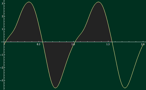
But what I find interesting is the dependence on the date or seasons, i.e. the fractional part of the year \(y\). My nonlinear fit was a general Fourier expansion up to the 6th higher harmonics – 12 coefficients in total (six for cosines, six for sines). For your convenience, here are two cycles of the cosine/sine part of the fit:

Apologies that the last, negative half-wave isn't filled black. I don't want to spend hours with similar things. The shape of the curve hasn't substantially changed when I added the 6th harmonic cosines and sines. But you see that it dramatically deviates from a simple shifted sine. It's a rather complicated curve. Incidentally, I have checked that I was visually unable to see the difference between the seasonal curve (fit) extracted from the first 20 years of Mauna Loa and the last 20 years of the dataset.
A naive person could think that the Northern and Southern hemispheres should cancel and there shouldn't be a difference between springs and autumns. However, that's wrong because what's primarily responsible for the seasonal variations are life processes on land and the land masses are mostly on the Northern Hemisphere (Eurasia and North America are large). So the graph pretty much emulates what the Northern Hemispheres wants to do to the CO2 while our friends in Australia and Antarctica are just negligible parrots, penguins, and kangaroos who are emulating what we're doing half a year later. ;-)
During winter, the plants – the players that are capable of absorbing CO2 – are losing their vitality and activity so the CO2 is increasing up to the maximum near 3.12 ppm (plus the long-term running average) for \(x\in 0.36+\ZZ\) – something like May 10th. That's where the trend is reverted and Northern Hemisphere plants start to blossom and absorb more CO2 than the annual average. That's why the CO2 drops up to the minimum around –3.58 ppm (plus the long-term running average) for \(x\in 0.74+\ZZ\), something like September 27th. Then the seasonal CO2 anomaly starts to go up again, and so on.
What I also find interesting is the slight "hole" near \(x\in 0.15+\ZZ\). The graph really refuses to be smooth at that point. Also, you may notice that \(0.74-0.36=0.38\) is substantially less than \(0.5\) which means that the decrease of CO2 during the Northern summers is faster than the increase of CO2 in the rest of the year. In other words, when plants start to boom and consume CO2, they may do so more quickly and efficiently than when they're failing to boom. ;-)
The latest reading is 396.74 from February 10th, 2013. In 2013, this is bound to increase by 3.6 ppm or so by May 10th or so. In other words, the maximum of Mauna Loa CO2 for 2013 in May will slightly exceed 400 ppm for the first time around mid May – about 400.3 ppm will be the annual maximum. I guess that we will hear about it again. If the alarmists weren't preparing this story for May 2013 yet, one of them who is a TRF reader at the same moment will surely steal the idea from your humble correspondent!
The sine-and-cosine part of the fit (see the last graph with two cycles) vanishes around January 8th and July 20th which are the dates for which the actual measured concentrations may be interpreted as the "long-term running means" with the seasonal variations removed. On July 22nd, 2012, they had 393.98 pm. On January 6th, 2013, it was 395.53 ppm. The latter is close to what we have "now" when the seasonal variations are suppressed.
Let me mention that between May and September, the seasonal variations contribute the drop by \(3.12+3.58=6.70\) ppm of CO2. If you could make plants thrive in the winter as well, you could easily subtract something like 13 ppm of CO2 from the atmosphere every year, well above the 2 ppm by which we are increasing the concentration every year (it's 1/2 of 4 ppm we are adding; the other half is already being absorbed by the enhanced consumption of CO2 due to the elevated concentrations).

Did you know that just 6,500 years ago, Britain was connected to Europe in this way? The British Euroskeptics were weaker than today. Hunters were working hard in the land just in between Britain and Denmark. On Wednesday night, I didn't want to believe those claims – I was imagining that the author of the story was envisioning some huge continental drift in just thousands of years ;-) – but when you think about it, it's completely natural that there had to be a land, Doggerland, because big chunks of the Northern Sea are extremely shallow, around 30 meters, and the sea level jumped by more than 100 meters in the last 20,000 years as the continental ice sheets melted.
During the next ice age, sometimes around 60,000 AD, Doggerland could become a land again. It would be fun to know what kind of people (or creatures) will be living there and in what way they will be communicating. Alternatively, we may rebuild Doggerland by landfills and other constructions much earlier, perhaps in 2020 AD.


Mauna Loa, one of the five volcanoes underlying Hawaii, a middle Pacific state of the U.S., is the most standardized place where the concentration is measured. See this NOAA page on Mauna Loa weekly and the raw data I have used.
If you open the page with the raw data, you will get over 2,000 weekly concentrations of carbon dioxide in ppmv (parts per million of volume – or equivalently, parts per million of the number of molecules) between May 1974 and February 2013. The page usefully offers you the decimal year. For example, February 10th, 2013 is written as \[
2013.1110 = 2013+\frac{40.5}{365}
\] because February 10th is the 41st day of the year with 365 days and the 41st day is offset by the average between 40 (number of days before it) and 41 (the ID). Think about it, it's natural: the extra one-half labels the noon, the middle of the day. The next step is to ignore the historical data and the entries –999.99 for the concentrations.
I did various things but the most important result I want to show you is a nonlinear fit for the concentration as a function of \(y\), the year that includes the fractional part remembering the date. Note that in the past, I offered you my "exponentially increasing" formula for the carbon dioxide concentration as a function of the year, ignoring the date – the seasonal variation:\[
c = 280 + 22.3 \exp\left(\frac{{\rm year}-1920}{57}\right)
\] However, we want to include the seasonally oscillating part of the graph. The following nonlinear fit is self-explanatory; all the "complicated" real numbers in it (280 isn't one of them) were optimized by the NonlinearModelFit command in Mathematica.\[
\eq{
{\rm conc}(x) &= 280 + \exp(4.359 + 0.02088 x)\\
&- 0.8263 \cos[2\pi x] + \\
&+ 0.6033 \cos[4\pi x] + 0.0255 \cos[6\pi x] - \\
&- 0.0208 \cos[8\pi x] + 0.0166 \cos[10\pi x] - \\
&- 0.0135 \cos[12\pi x] + \\
&+ 2.8359 \sin[2\pi x] - \\
&- 0.5413 \sin[4\pi x] - 0.0957 \sin[6\pi x] + \\
&+ 0.0430 \sin[8\pi x] + 0.0218 \sin[10\pi x] - \\
&- 0.0002 \sin[12\pi x],\\
\\
x &= y - 1994.
}
\] Sorry, for the strange brackets and other imperfections of the \(\rm \LaTeX\). You see that the base concentration was chosen to be 280 ppm and the increase was prescribed to be exponential. In the exponent, the slope is\[
0.0208774 = 1/47.899
\] so the \(e\)-folding time seems to be shorter than those 57 years that are optimal for the interpolation from the beginning of the Industrial Revolution. You could say that according to the 1974-2013 data, it seems that the time in which the CO2 excess above 280 ppm gets multiplied by \(e=2.718\dots\) is shorter than 50 years. Roughly speaking, the same thing holds for the annual emissions. Here is the 1974-2014 graph.

But what I find interesting is the dependence on the date or seasons, i.e. the fractional part of the year \(y\). My nonlinear fit was a general Fourier expansion up to the 6th higher harmonics – 12 coefficients in total (six for cosines, six for sines). For your convenience, here are two cycles of the cosine/sine part of the fit:
Apologies that the last, negative half-wave isn't filled black. I don't want to spend hours with similar things. The shape of the curve hasn't substantially changed when I added the 6th harmonic cosines and sines. But you see that it dramatically deviates from a simple shifted sine. It's a rather complicated curve. Incidentally, I have checked that I was visually unable to see the difference between the seasonal curve (fit) extracted from the first 20 years of Mauna Loa and the last 20 years of the dataset.
A naive person could think that the Northern and Southern hemispheres should cancel and there shouldn't be a difference between springs and autumns. However, that's wrong because what's primarily responsible for the seasonal variations are life processes on land and the land masses are mostly on the Northern Hemisphere (Eurasia and North America are large). So the graph pretty much emulates what the Northern Hemispheres wants to do to the CO2 while our friends in Australia and Antarctica are just negligible parrots, penguins, and kangaroos who are emulating what we're doing half a year later. ;-)
During winter, the plants – the players that are capable of absorbing CO2 – are losing their vitality and activity so the CO2 is increasing up to the maximum near 3.12 ppm (plus the long-term running average) for \(x\in 0.36+\ZZ\) – something like May 10th. That's where the trend is reverted and Northern Hemisphere plants start to blossom and absorb more CO2 than the annual average. That's why the CO2 drops up to the minimum around –3.58 ppm (plus the long-term running average) for \(x\in 0.74+\ZZ\), something like September 27th. Then the seasonal CO2 anomaly starts to go up again, and so on.
What I also find interesting is the slight "hole" near \(x\in 0.15+\ZZ\). The graph really refuses to be smooth at that point. Also, you may notice that \(0.74-0.36=0.38\) is substantially less than \(0.5\) which means that the decrease of CO2 during the Northern summers is faster than the increase of CO2 in the rest of the year. In other words, when plants start to boom and consume CO2, they may do so more quickly and efficiently than when they're failing to boom. ;-)
The latest reading is 396.74 from February 10th, 2013. In 2013, this is bound to increase by 3.6 ppm or so by May 10th or so. In other words, the maximum of Mauna Loa CO2 for 2013 in May will slightly exceed 400 ppm for the first time around mid May – about 400.3 ppm will be the annual maximum. I guess that we will hear about it again. If the alarmists weren't preparing this story for May 2013 yet, one of them who is a TRF reader at the same moment will surely steal the idea from your humble correspondent!
The sine-and-cosine part of the fit (see the last graph with two cycles) vanishes around January 8th and July 20th which are the dates for which the actual measured concentrations may be interpreted as the "long-term running means" with the seasonal variations removed. On July 22nd, 2012, they had 393.98 pm. On January 6th, 2013, it was 395.53 ppm. The latter is close to what we have "now" when the seasonal variations are suppressed.
Let me mention that between May and September, the seasonal variations contribute the drop by \(3.12+3.58=6.70\) ppm of CO2. If you could make plants thrive in the winter as well, you could easily subtract something like 13 ppm of CO2 from the atmosphere every year, well above the 2 ppm by which we are increasing the concentration every year (it's 1/2 of 4 ppm we are adding; the other half is already being absorbed by the enhanced consumption of CO2 due to the elevated concentrations).
Did you know that just 6,500 years ago, Britain was connected to Europe in this way? The British Euroskeptics were weaker than today. Hunters were working hard in the land just in between Britain and Denmark. On Wednesday night, I didn't want to believe those claims – I was imagining that the author of the story was envisioning some huge continental drift in just thousands of years ;-) – but when you think about it, it's completely natural that there had to be a land, Doggerland, because big chunks of the Northern Sea are extremely shallow, around 30 meters, and the sea level jumped by more than 100 meters in the last 20,000 years as the continental ice sheets melted.
During the next ice age, sometimes around 60,000 AD, Doggerland could become a land again. It would be fun to know what kind of people (or creatures) will be living there and in what way they will be communicating. Alternatively, we may rebuild Doggerland by landfills and other constructions much earlier, perhaps in 2020 AD.
23 February 2013
15 February 2013
13 February 2013
11 February 2013
10 February 2013
06 February 2013
02 February 2013
01 February 2013
Subscribe to:
Posts (Atom)